Example analysis

library(tjdc)
library(dplyr)
library(tidyr)
library(posterior)
library(ggplot2)
library(sf)

theme_set(theme_bw())

Data

Use the internal example, which is a datacube with clear blocks of changepoints.

data("easystripes")

x <- easystripes$strip
# the truth
j <- easystripes$jump
# as data frame
xdf <- tj_stars_to_data(x) 
jdf <- as_tibble(j) |> rename(c_x = x, c_y = y, jump_after = values)

# add truth
df  <- xdf |> 
  left_join(  jdf   )
#> Joining with `by = join_by(c_x, c_y)`

# Some examples
df_ex <- df |> 
  group_by(jump_after) |> 
  filter( cell %in% sample(unique(cell), 30) )

This datacube has $T=11$ timepoints, and a clear structure of where the changes take place.

plot( x )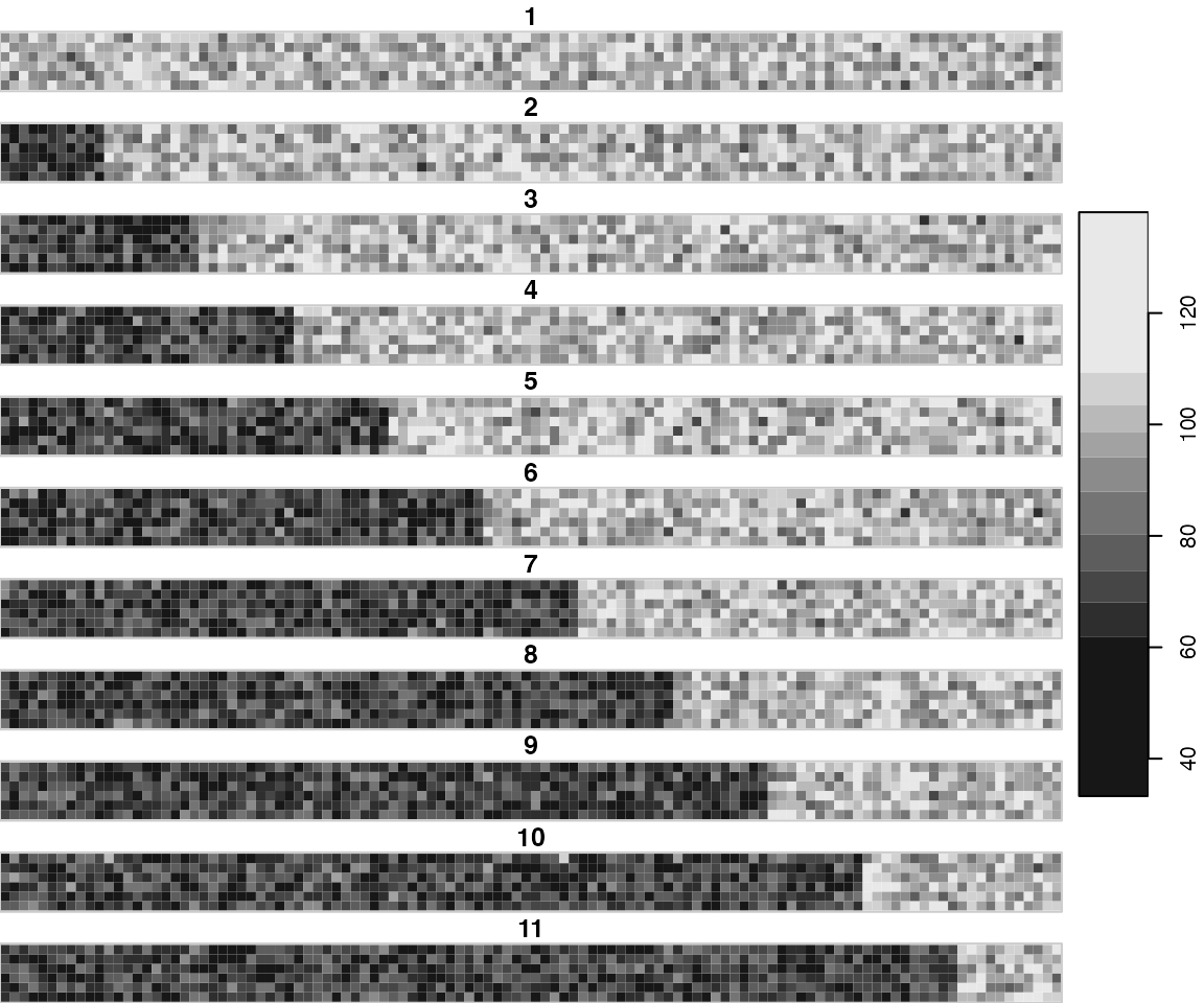

Here are examples of the series with different changepoints. Note that jumping after $t=11$ is the same as not having a changepoint.

df_ex |> 
  ggplot() +
  geom_line(aes(time, value, group = cell)) +
  facet_wrap(~jump_after)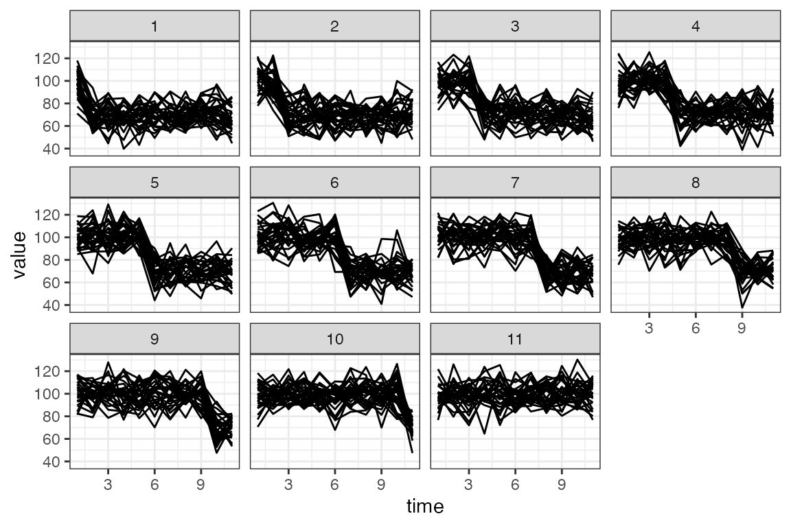

Fit the model

The most up-to-date fitting function is at the moment called tj_fit_m0.6

# set prior: negative jumps only.
p_d <- list(m = 0, s2 = 1e4, a = -Inf, b = 0)

fit0 <- tj_fit_m0.6(x, 
                     prior_k = 0.9,
                     niter = 1000,
                     prior_delta = p_d,
                     verbose = TRUE)

By default,

• The pixel-to-pixel ‘correlation’ term $\gamma=0$ so no spatial interaction is set (see gamma)
• The priors are pretty flat
  • see prior_theta for the linear model parameters (2D Gaussian i.i.d. over pixels)
  • see prior_delta for the jump-size parameter, (1D truncated Gaussian i.i.d. over pixels)
  • see prior_sigma2 for residual variance (Gamma, one for all pixels)
  • see prior_k the prior probability of jumps; $T$-vector or 1 value for $1-P(no~jump)$
• all of the MCMC traces are kept in the output (see keep_hist parameter in the help).

The proposed model is activated by setting $\gamma\neq 0$:

fit1 <- tj_fit_m0.6(x, 
                     gamma = 0.6,
                     prior_k = 0.9,
                     niter = 1000,
                     prior_delta = p_d,
                     verbose = TRUE)

There are many components in the result object, but most importantly the posteriors are in

• k: The posterior probabilities for a jump, in format k[t,i]. So for example, the probability of no jump of pixel 2 when $T=11$ is in k[11,2]. The probability of a jump somewhere is also returned in component z
• theta_m, theta_Suppetri: The posterior mean and (upper triangle of) covariance for the vector $(\theta,\delta)$ (regression + jump)
• sigma2: Residual variance
• traces start with hist_, e.g. hist_z, hist_sigma2

Example: Check convergence.

# example cell:
c <- 123
tr <- cbind(fit1$hist_theta[,c,],
            fit1$hist_z[,c],
            fit1$hist_sigma2) |> 
  as.data.frame() |>  
  setNames(c("a", "b", "d", "P(jump)", "sigma2"))

# use `posterior` etc.
trp <- as_draws(tr[-(1:500),])
summary( trp )
#> # A tibble: 5 × 10
#>   variable    mean  median     sd      mad      q5    q95  rhat ess_bulk
#>   <chr>      <dbl>   <dbl>  <dbl>    <dbl>   <dbl>  <dbl> <dbl>    <dbl>
#> 1 a         96.7    96.7   10.5   9.43e+ 0  78.5   114.   1.05      33.1
#> 2 b          0.261   0.240  1.07  1.03e+ 0  -1.52    1.98 1.00     125. 
#> 3 d        -30.4   -27.6   17.2   1.07e+ 1 -52.8   -13.0  1.01      41.6
#> 4 P(jump)    0.971   1      0.161 1.65e-16   0.983   1    1.04      23.4
#> 5 sigma2   104.    104.     1.99  2.03e+ 0 101.    107.   0.999    281. 
#> # ℹ 1 more variable: ess_tail <dbl>

tr |> 
  mutate(iter = 1:n()) |> 
  pivot_longer(-iter)  |> 
  ggplot() +
  geom_line(aes(iter, value)) +
  facet_wrap(~name, scale = "free_y")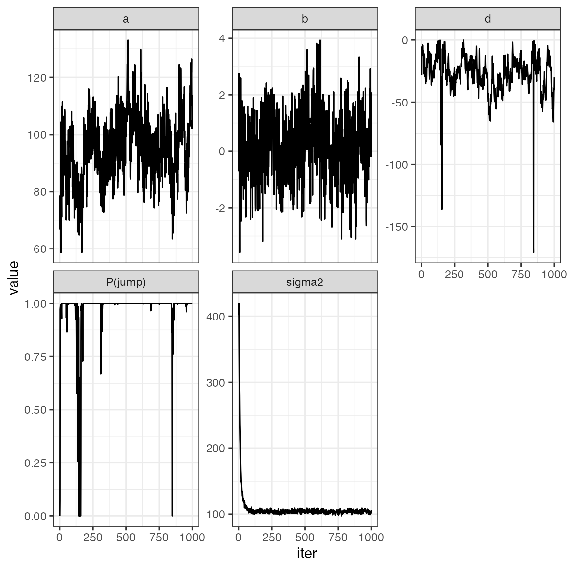

Example: get the most likely jump times.

pk0_most_likely <- apply(fit0$k, 2, which.max)
pk1_most_likely <- apply(fit1$k, 2, which.max)
pk0df           <- fit0$cell_info |> mutate(jump_after = pk0_most_likely)
pk1df           <- fit1$cell_info |> mutate(jump_after = pk1_most_likely)

Compare to truth:

# Gather estimates
df_o <- bind_rows(pk0df |> mutate(model = "cell-to-cell correlation/interaction"),
                  pk1df |> mutate(model = "cell-to-cell interaction"),
                  df    |> filter(time == 1) |> mutate(model = "truth")) |> 
  mutate(est = factor(jump_after))

# pretty color
cc <- c(hcl.colors(10, palette = "PuOr"), "black")

# Plot
df_o |> 
  ggplot() +
  geom_raster(aes(c_x, c_y, fill = est), show.legend = FALSE) +
  coord_fixed(expand = FALSE) +
  scale_fill_manual(values = cc ) +
  facet_wrap(~model, ncol = 1)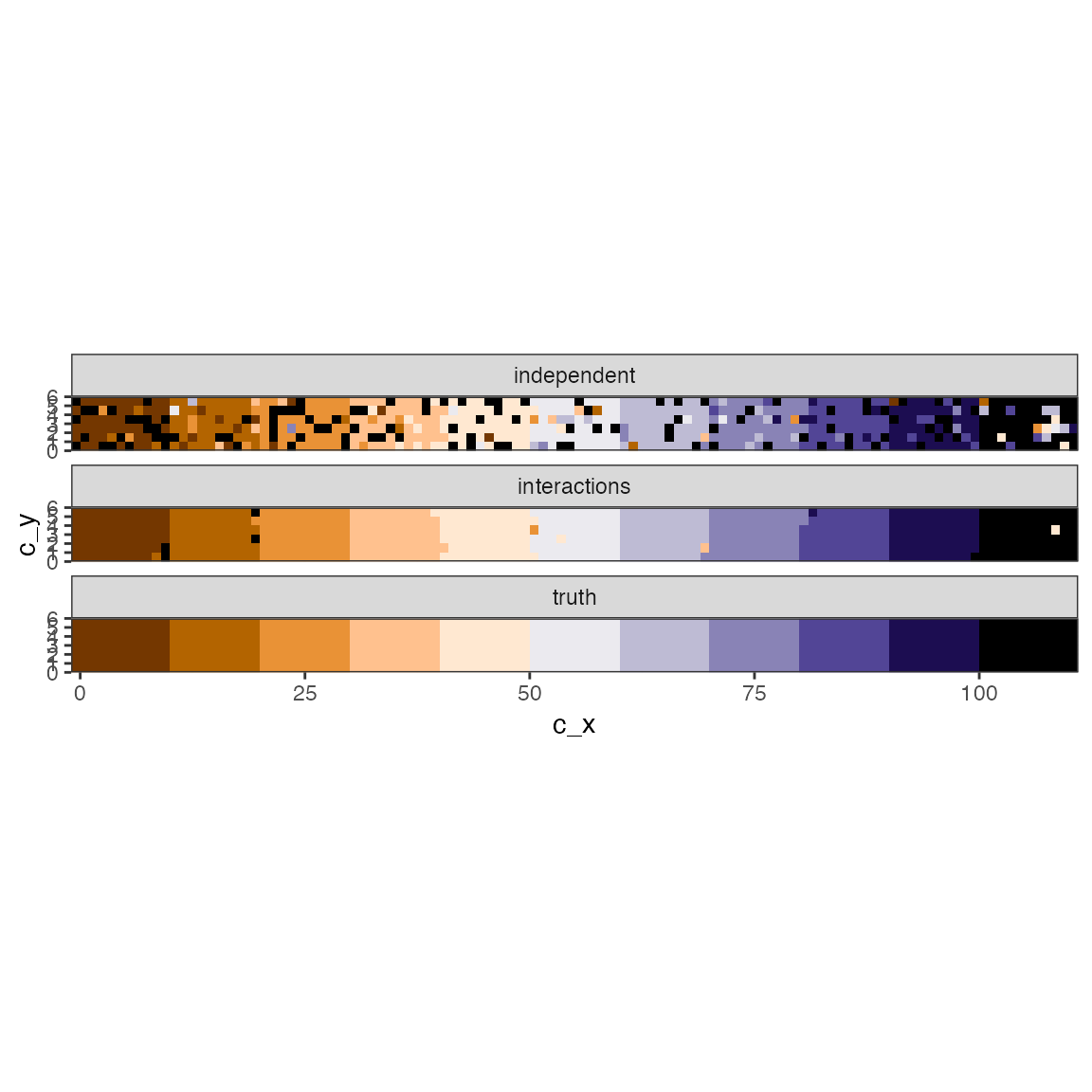

Naive parallelisation

Large dimension cube can be split into smaller cubes at the spatial domain (raster), and model fitted to each subset separately and independently, facilitating simple parallelisation. Due to the spatial dependency structure, it is a good idea to overlap the regions a bit. There are three useful functions here:

1. tj_divide_raster: Create the geometry of the subsets
2. tj_fit_m0.x: Fit a model to each subset, and handle collection and possible storage writing
3. tj_stitcher_m0.x: Collect the results.

First we want to create the mosaic.

tiling <- tj_divide_raster(x, n = c(3, 1), buffer = c(1, 1))

The result contains info on the tiling. For example, sf polygons of the tiles are available.

tiling$poly |> 
  ggplot() + 
  geom_sf( data = st_bbox(x) |> st_as_sfc() , fill = "orange") + 
  geom_sf(alpha = .5) +
  geom_sf_text(aes(label = id)) +
  expand_limits(y = c(-2, 8) )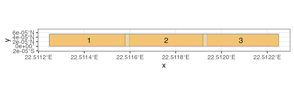

Here we have split the raster bounding box into $3$-columns-$1$-rows separate boxes, with overlap of 2 pixels.

Then we use the wrapper to fit the model on each subset.

fitm_l <- tj_fit_m0.x(x, 
                    timevar = "z",
                    tiling = tiling,
                    niter = 1000,
                    prior_k = 0.9,
                    gamma = .6, 
                    prior_delta = p_d,
                    model_variant = "m0.6",
                    ncores = 3)
#> [m0.x 3c][1/1][ave time 4.796938 secs, -0.00021 secs left, ready 2025-10-10 08:07:21]     
#> [m0.x 3c][1/1][ave time 4.796938 secs][total time: 4.798993 secs]

By default all stuff is kept in memory. See the documentation on how to store each fit into custom file location.

The result is a list of fits, and needs to be parsed together, particularly the pixels in the overlapping sections need to be made unique.

# parse the results from separate tiles
fitm <- tj_stitcher_m0.x(fitm_l, tiling)

Which has a structure similar to the earlier estimate with the full data.

pkm_most_likely <- apply(fitm$k, 2, which.max)

pkmdf <- fitm$cell_info |> 
  # this table contains duplicate rows for cells in the overlaps
  group_by(cell) |> 
  filter(row_number() == 1) |> 
  ungroup() |> 
  left_join( 
    tibble( cell = fitm$cells, jump_after = pkm_most_likely )  )
#> Joining with `by = join_by(cell)`
  

# Gather estimates
df_o2 <- bind_rows(pk1df |> mutate(model = "full"),
                   pkmdf |> mutate(model = "in parts") ) |> 
  mutate(est = factor(jump_after))

# Plot
df_o2 |> 
  ggplot() +
  geom_raster(aes(c_x, c_y, fill = est), show.legend = FALSE) +
  coord_fixed(expand = FALSE) +
  scale_fill_manual(values = cc ) +
  facet_wrap(~model, ncol = 1)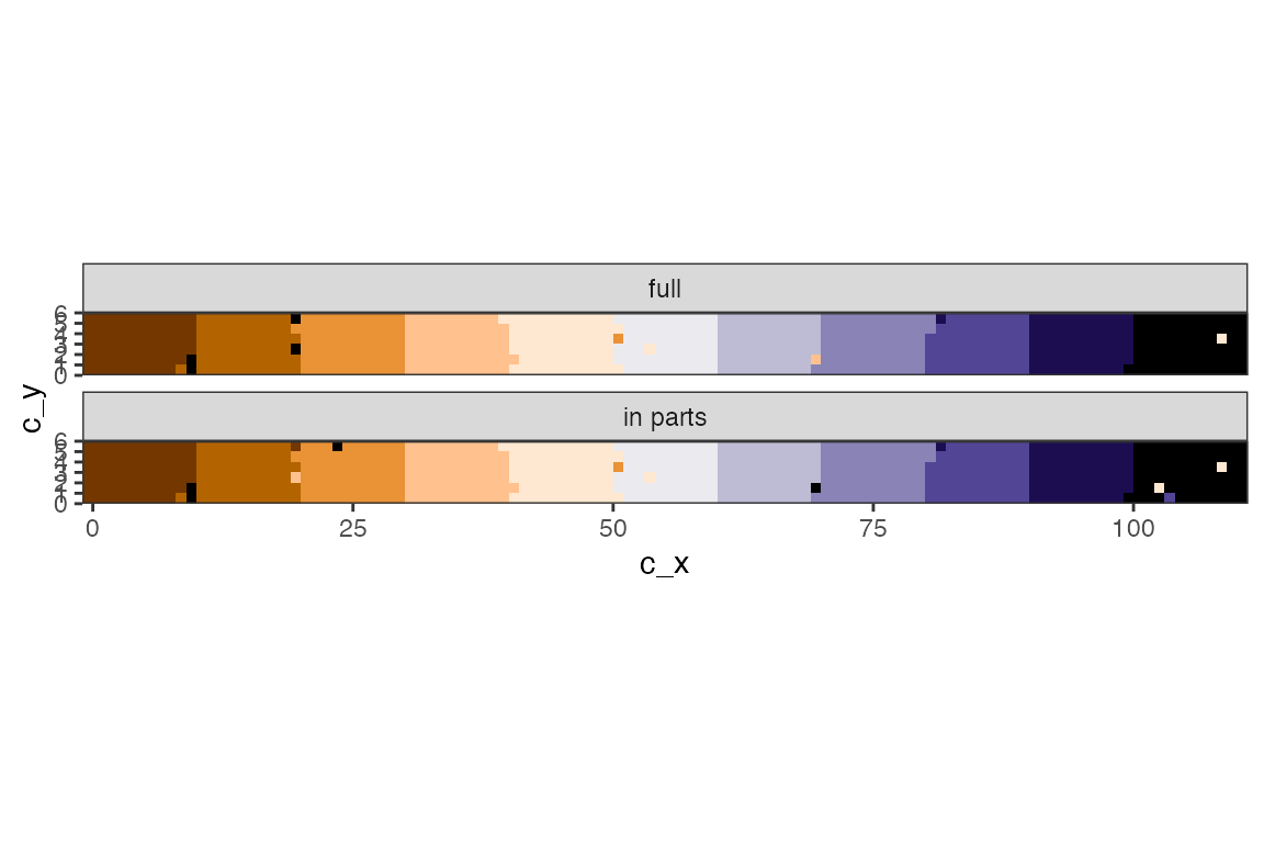 

Note that for parallel fits the variance parameters will be estimated separately.

s2 <- fitm$hist_sigma2 |> as_draws()
colnames(s2) <- paste0("sigma2_", 1:3)
summary(s2)
#> # A tibble: 3 × 10
#>   variable  mean median    sd   mad    q5   q95  rhat ess_bulk ess_tail
#>   <chr>    <dbl>  <dbl> <dbl> <dbl> <dbl> <dbl> <dbl>    <dbl>    <dbl>
#> 1 sigma2_1  107.   105.  20.1  3.54  99.0  114.  1.03     37.0     12.6
#> 2 sigma2_2  111.   107.  29.3  3.97 102.   119.  1.03     45.9     10.7
#> 3 sigma2_3  105.   101.  27.5  3.49  95.7  108.  1.02    131.      34.8

Time comparison:

c(full = fit1$took,
  in_parts = fitm$took)
#> Time differences in secs
#>      full  in_parts 
#> 12.427528  4.604832