Example 2D anisotropy analysis using Kdirectional

Originally written around 2014. Updated 10.12.2022.

Introduction

The package Kdirectional is a collection of tools for analysing the isotropy of 2- and 3-dimensional point patterns. This document shows how to use some of these tools by analysing an synthetic example pattern.

In this vignette we use the following packages:

library(spatstat)
library(Kdirectional)

Example pattern

We simulate Strauss process and transform it. Assume the transformation is

comp <- 0.7
D <- diag( c(comp, 1/comp))
angle <- pi/8
R <- rotationMatrix3(az=angle)[-3,-3] # internal, not rgl one
C <- R%*%D

that is, we compress the x-axis by factor 0.7 and stretch the y-axis to keep volume 1. Then we simulate the original process in a window that will be square after the transformation

set.seed(1)
x0 <- rStrauss(500, gamma = 0.05, R = 0.03, W = affine(square(), solve(C)))

and transform it to the observed pattern

x <- affine(x0, C)

Check things went ok (define a little helper for plotting):

plotp <- function(...) plot(..., cex=.3)
par(mfrow=c(1,2), mar=c(1,1,1,1))
plotp(x0)
plotp(x)

The pattern on the left is what we want to estimate.

Nearest neighbour vectors

Check for starters the distribution of nearest neighbours vectors.

nna <- nnangle(coords(x))
ang <- nna[,1]-pi
par(mfrow=c(1,2))
angles.flower(ang, ci = T, k=24, bty = "n")
# Compare to spatstat
rose(ang, unit = "rad", nclass = 24+1, main = "")

The blue rings give approximate 95% pointwise confidence intervals. Hard to see anything definite, perhaps some peakyness at the 2:30’oclock axis. Nearest neighbours are not very informative, so let’s analyse the full set of pairwise vectors.

Fry-points and ellipsoids

As in the paper [1], the Fry-points tell us interesting things about the isotropy.

f <- fry_ellipsoids(x, nvec=1:20, nangles = 30, eps=0.1, r_adjust = .2)

r_adjust=.2 reduces the computations to pairs with length within 20% window width, eps adds a bit of angular smoothing (in radians), and nangles chooses the amount of directions to look at.

Plot the estimated ellipsoids:

plot(f, zoom=.3, used_points = FALSE)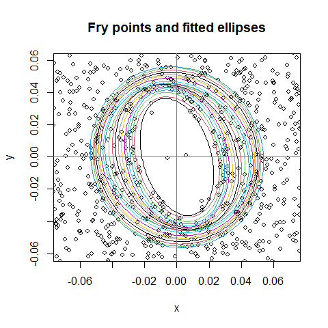

Oval shape is visible, some ambiguity of rotation. Check the ellipticity with a contrast \(axis_x-axis_y=0\):

ci <- confint(f, nsim=500)
print(summary(ci)[1:5,], digits=2)

##           mean  median sd     CI.2.5% CI.97.5% p     
## Contour_1 0.014 0.015  0.034  -0.048  0.11     0.68  
## Contour_2 0.015 0.014  0.0053 0.0054  0.026    0.01  
## Contour_3 0.015 0.015  0.0053 0.0056  0.027    0.0074
## Contour_4 0.016 0.016  0.0066 0.0048  0.031    0.02  
## Contour_5 0.017 0.016  0.0084 0.0014  0.035    0.055

plot(ci, ylim = c(-1,1)*.1)

The first contour is poorly estimated as there are some short range pairs, kind of like Poisson noise. Others seem to hint of compression (the p-values and confidence intervals are biased and conservative).

Let’s compute the average rotation, where we scale each ellipsoid to have det = 1 by setting just_rotation=TRUE.

contours <- f$ellipsoids[-1]
mean_e <- mean_ellipsoids(contours, just_rotation = TRUE)
summary(mean_e)

## Average 2D ellipse, computed from 19 2D ellipses.
## 
## Estimates:
##  Center:       (-0.003603507,  0.033050560)
##  Semi-axes lengths (absolute):     0.906708 : 1.113431 
##  Semi-axes lengths (relative):     1.000 : 1.228 
##  Rotation angles (rad):    -2.768 
##  Rotation angles (deg):    -158.6 
##  Error variance:       0.007447662

Rotation seems to be non-zero (or non \(\pm\pi\)). Ignore the error variance, its not correct.

c(true=angle, est=mean_e$rot_angle + pi)

##      true       est 
## 0.3926991 0.3739214

Backrotate the pattern:

Rhat <- rotationMatrix3(az=pi)[-3,-3]%*%mean_e$rot 
xr <- affine(x, solve(Rhat))

Next we estimate the compression by minimizing the difference of K-functions along the main axes. We need to provide a grid to optimise over:

gamma_vec <- seq(0.5, 1, by=0.05)
grid <- cbind(gamma_vec, 1/gamma_vec)

Then compute the anisotropy profile:

r <- seq(0, 0.2, length=50)
eps <- pi/10
ani <- anisotropy_profile(xr, grid = grid, r=r, eps=eps, power=2)
ani0 <- anisotropy_profile(x, grid = grid, r=r, eps=eps, power=2)

We set the sector-K angle with eps and use integral of squared differences (power=2) as the distance.

Plot the profiles, scaled to 0-1 for plotting (it’s the default):

plot(ani, type="b", scale=TRUE)
lines(ani0, type="b", col=2)

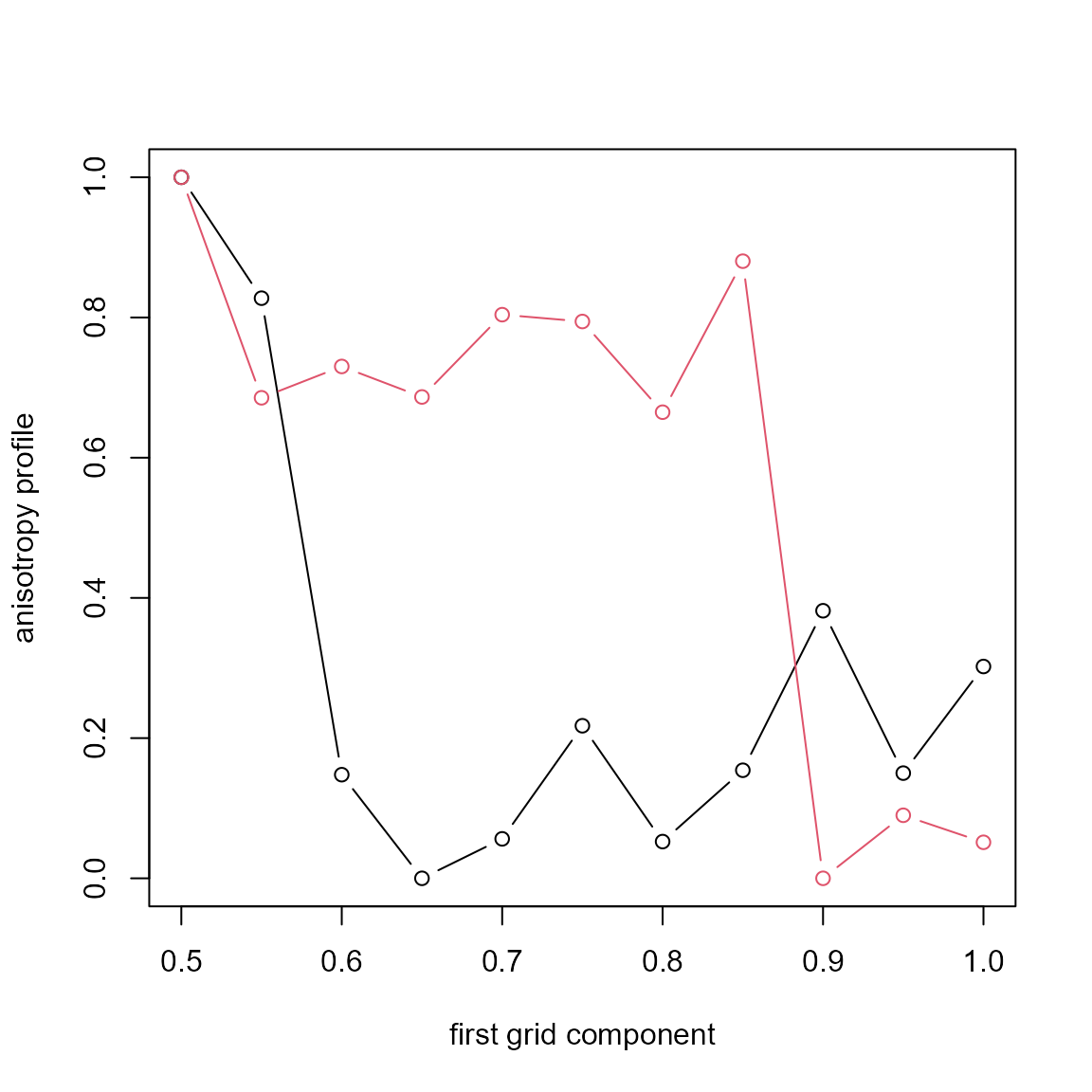
( s <- summary(ani) )

## Anisotropy profile
## Range of integration: [ 0 , 0.2 ]
## Difference power: 2 
## Optimal transformation: diag( 0.65 1.538462 )

Estimated compression

c(true=comp, est=s$estimate[1])

## true  est 
## 0.70 0.65

Backtransform:

Dhat <- s$estimate
xhat <- affine(xr, solve(Dhat))

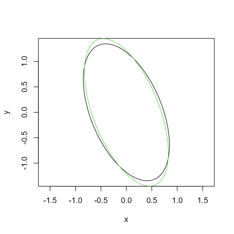
Recap of the steps:

par(mfrow=c(2,2), mar=c(1,1,1,1))
plotp(x)
plotp(xr)
plotp(xhat)
plotp(x0)

Finally, let’s illustrate the estimated transformation. Use simulation and estimation to get an ellipsoid object:

Chat <- Rhat %*% Dhat
e0 <- ellipsoid_OLS( rellipsoid(1000, c(1,1), R = C) )
e <- ellipsoid_OLS( rellipsoid(1000, c(1,1), R = Chat) )

plot(e0, add=FALSE)
plot(e, col=3)

References

[1] T Rajala, A Särkkä, C Redenbach, M Sormani (2015): Estimating geometric anisotropy in spatial point patterns, Spatial Statistics

Tuomas Rajala

2022-12-10

Introduction

Example pattern

Nearest neighbour vectors

Fry-points and ellipsoids

References